[1]:
%load_ext autoreload
%autoreload 2
[2]:
import os

os.environ["XLA_PYTHON_CLIENT_PREALLOCATE"] = "false"
os.environ["CUDA_VISIBLE_DEVICES"] = ""

import jax
import jax.numpy as jnp
import matplotlib.pyplot as plt
import numpy as np
import time

from phentax.waveform import IMRPhenomTHM

from lisaconstants import ASTRONOMICAL_YEAR

FIGSIZE = (10, 6)
import scienceplots
plt.style.use(["science", "notebook"])
Phentax basic tutorial
First, create the waveform generator.
Here we create all the allowed higher modes. The first step is initialize the waveform generator with the desired settings:
[3]:
tlowfit = True # use a fit to set the starting time of the root finder used in t(f)
tol = 1e-12 # root finding tolerance
Tobs = 5 * ASTRONOMICAL_YEAR / 12

imr = IMRPhenomTHM(
        higher_modes="all",
        include_negative_modes=True, # negative m modes will be produced by simmetry
        t_low_fit=tlowfit,
        coarse_grain=False, # if false it will generate the waveform on a dense time grid with the specified timestep
        atol=tol,
        rtol=tol,
        T=Tobs,
    )
[4]:
imr
[4]:
IMRPhenomTHM(higher_modes=[21 33 44 55], include_negative_modes=True, coarse_grain=False, t_low=0.0, atol=1e-12, rtol=1e-12, T=13149229.068144)
generate amplitudes and phases for one single binary
Since we use jax.jit to speed up the waveform generation, we need to run it once to compile the code.
Run the next two cells twice to verify the difference in performance.
[5]:
m1 = 1e7
m2 = 5e6
chi1 = 0.9
chi2 = 0.3
distance = 500.0
inclination = jnp.pi / 3.0
phi_ref = 0.0
psi = 1.0
f_min = 1e-4
delta_t = 10
f_ref = f_min
# t_ref = 0.0
to ensure compatibility with JAX’s vmap functionality, every output has to have the same shape. For this reason, together with times and quantities of interest, we return a mask that for each binary indicates the valid time points.
[6]:
wf_params, times, mask, amplitudes, phases = imr.compute_amp_phase(
        m1,
        m2,
        chi1,
        chi2,
        distance,
        phi_ref,
        inclination,
        psi,
        delta_t=delta_t,
        f_min=f_min,
        f_ref=f_ref,
    )
With compute_amp_phase, we can compute the amplitudes and phases of all the positive-m modes at once. Negative-m modes can be obtained from the positive-m modes by symmetry.
[7]:
num_binaries, num_modes, num_times = amplitudes.shape
print(f"Number of binaries: {num_binaries}")
print(f"Number of modes: {num_modes}")
print(f"Number of time points: {num_times}")
Number of binaries: 1
Number of modes: 5
Number of time points: 1314923
We can access the entries of a specific mode by indexing the second dimension of the output arrays. For example, to access the \((l,m)\) mode, we can do:
[8]:
mode = (2, 1)
mode_idx = imr.get_mode_index(mode)
print(f"Index of mode {mode}: {mode_idx}") # should be 1

amplitude_mode, phase_mode = amplitudes[:, mode_idx, :], phases[:, mode_idx, :]
Index of mode (2, 1): 1
The overall list of modes included in the waveform can be accessed via the modes_list property:
[9]:
print(f"Modes included in the waveform: \n {imr.modes_list}")
Modes included in the waveform:
 [[ 2  2]
 [ 2  1]
 [ 3  3]
 [ 4  4]
 [ 5  5]
 [ 2 -2]
 [ 2 -1]
 [ 3 -3]
 [ 4 -4]
 [ 5 -5]]
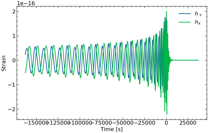
generate plus and cross polarizations for one single binary
[10]:
times, mask, h_plus, h_cross = imr.compute_polarizations_at_once(
        m1,
        m2,
        chi1,
        chi2,
        distance,
        phi_ref,
        inclination,
        psi,
        delta_t=delta_t,
        f_min=f_min,
        f_ref=f_ref,
    )
[11]:
fig = plt.figure(figsize=FIGSIZE)
plt.plot(times[mask], h_plus[mask], label=r"$h_+$")
plt.plot(times[mask], h_cross[mask], label=r"$h_x$")
plt.legend()
plt.xlabel("Time [s]")
plt.ylabel("Strain")
plt.show()
[12]:
# empty the memory allocated by jax
del times, mask, h_plus, h_cross
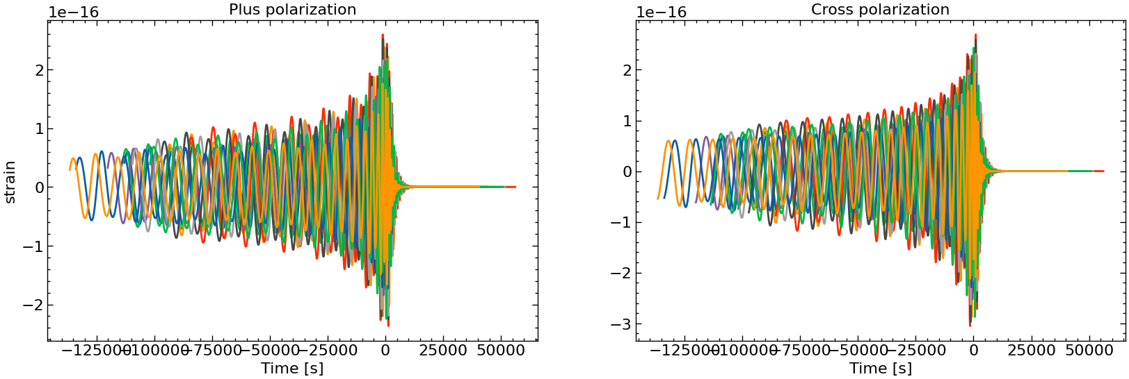
we can use the same logic and signature to generate a batch of waveforms.
For simplicity, here we add a random deviation from the previous parameters.
[13]:
key = jax.random.PRNGKey(0)
Since the input shape of our waveform’s parameters is now (batch_size,), we have to recompile the waveform function.
Again, run the next two cells twice to verify the difference in performance.
[14]:
num_binaries = 10
num_params = 8

key, subkey = jax.random.split(key)
random_params = jax.random.uniform(subkey, (num_binaries, num_params))

m1_batch = ( 1 + 0.7 * random_params[:, 0]) * m1
m2_batch = ( 1 + 0.5 * random_params[:, 1]) * m2
chi1_batch = (1 + 0.1 * random_params[:, 2]) * chi1
chi2_batch =  (1 + 0.1 * random_params[:, 3]) * chi2
distance_batch = (1 + 0.1 * random_params[:, 4]) * distance
phi_ref_batch = ( 1 + 0.1 * random_params[:, 5]) * phi_ref
psi_batch = ( 1 + 0.1 * random_params[:, 6]) * psi
inclination_batch = (1 + 0.1 * random_params[:, 7]) * inclination
[15]:
tic = time.time()

times_batch, mask_batch, h_plus_batch, h_cross_batch = imr.compute_polarizations_at_once(
        m1_batch,
        m2_batch,
        chi1_batch,
        chi2_batch,
        distance_batch,
        phi_ref_batch,
        inclination_batch,
        psi_batch,
        delta_t=delta_t,
        f_min=f_min,
        f_ref=f_ref,
        T = 3 / 12 * ASTRONOMICAL_YEAR
    )

h_plus_batch.block_until_ready()
print(f"Time elapsed: {time.time() - tic} s")
Time elapsed: 11.360782146453857 s
The compilation is needed only when the shape of the input arrays changes.
The dimension along the time axis of the waveform is given by the observation time T.
This allows to avoid the need of recompiling the internal functions when the required duration changes with the mass.
[16]:
h_plus_batch.shape
[16]:
(10, 788954)
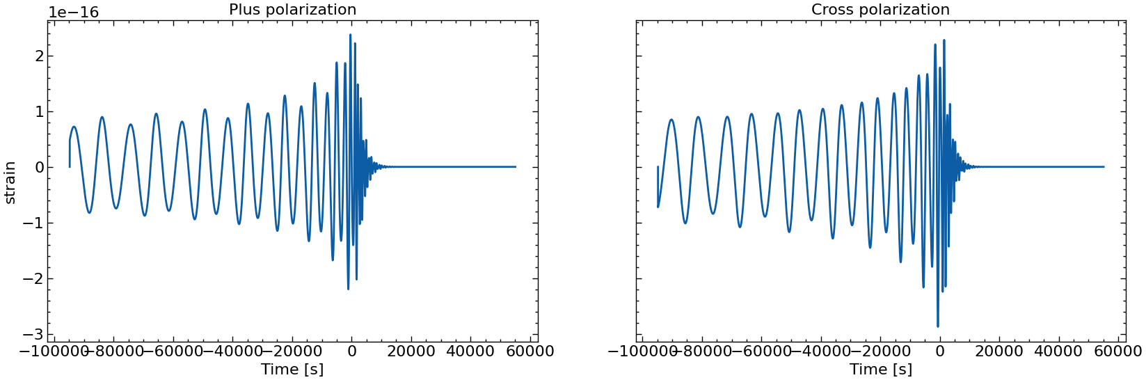
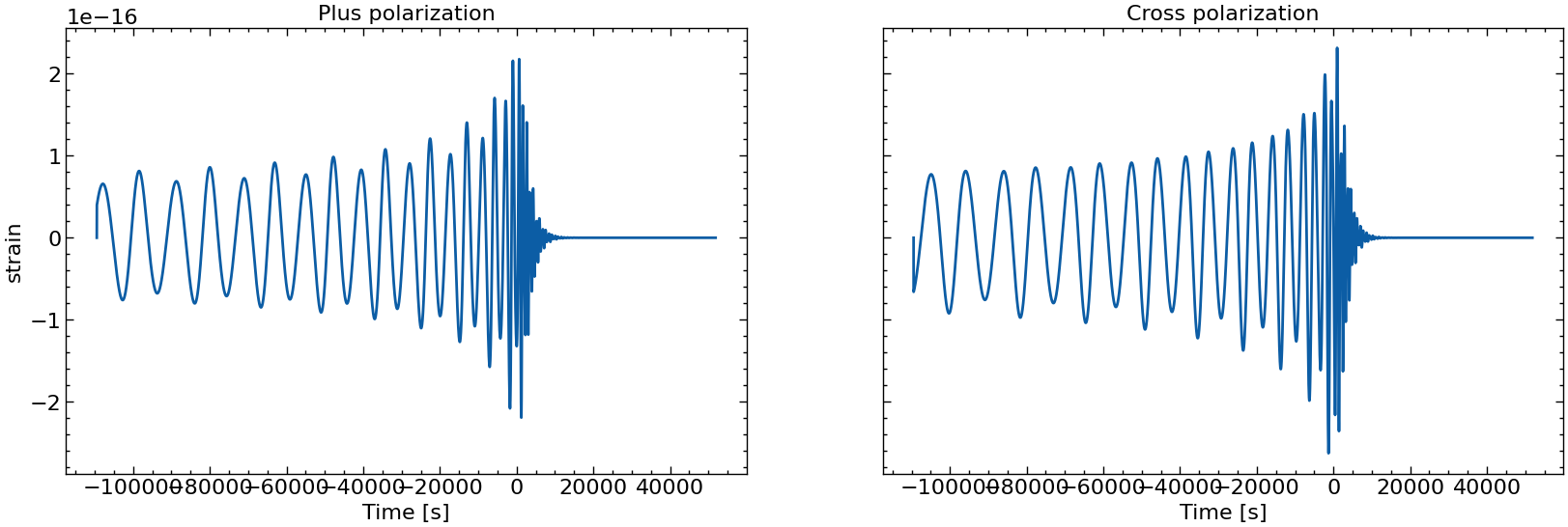
[17]:
# plot all the polarizations
fig, axs = plt.subplots(1, 2, figsize=(2 * FIGSIZE[0], FIGSIZE[1]))
for i in range(10):
    axs[0].plot(times_batch[i][mask_batch[i]], h_plus_batch[i][mask_batch[i]])
    axs[1].plot(times_batch[i][mask_batch[i]], h_cross_batch[i][mask_batch[i]])

axs[0].set_title("Plus polarization")
axs[1].set_title("Cross polarization")
#plt.legend()
axs[0].set_xlabel("Time [s]")
axs[1].set_xlabel("Time [s]")
axs[0].set_ylabel("strain")
plt.show()
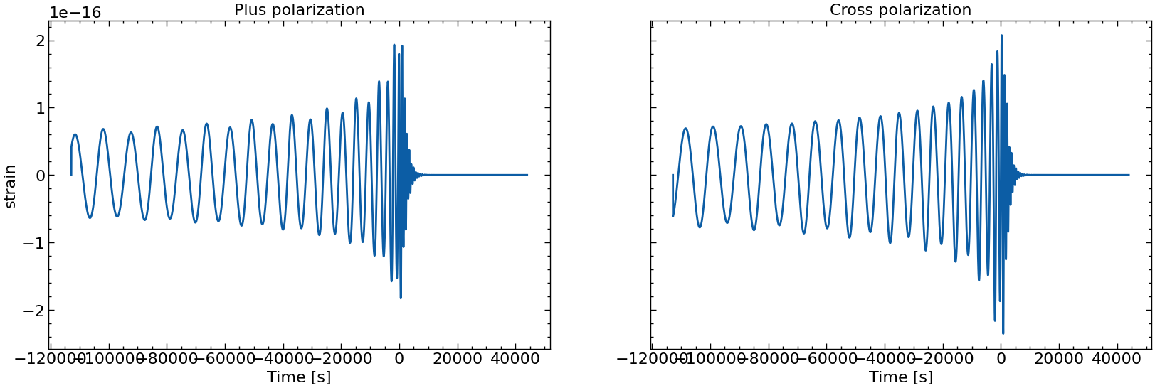
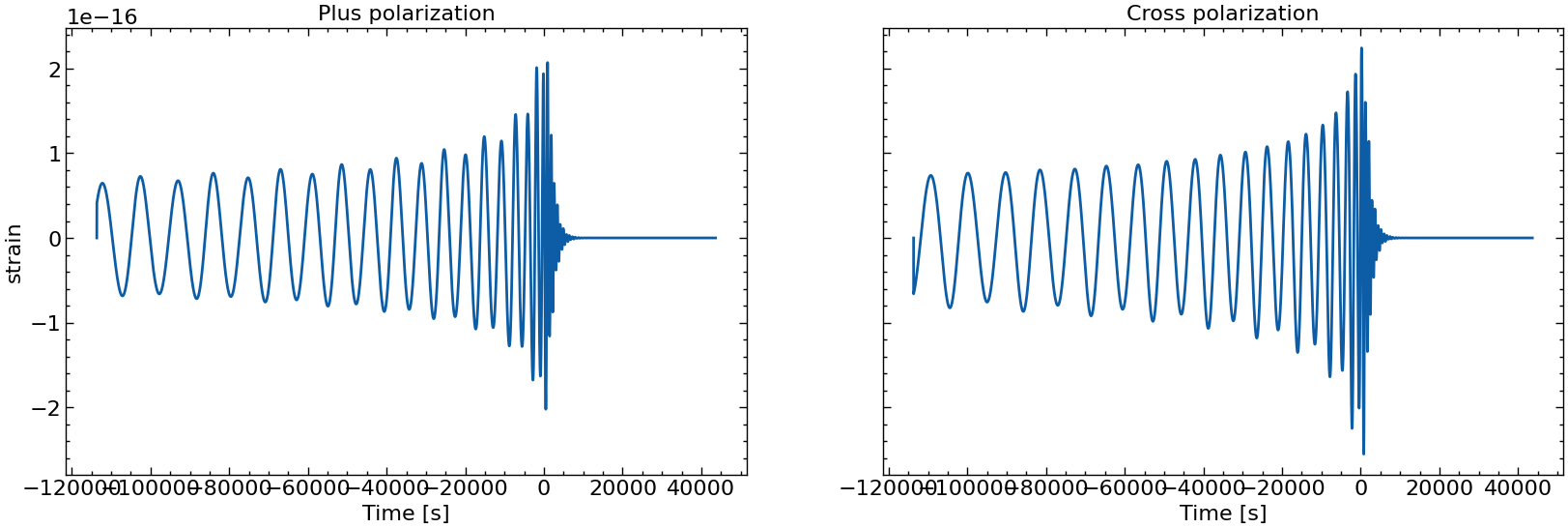
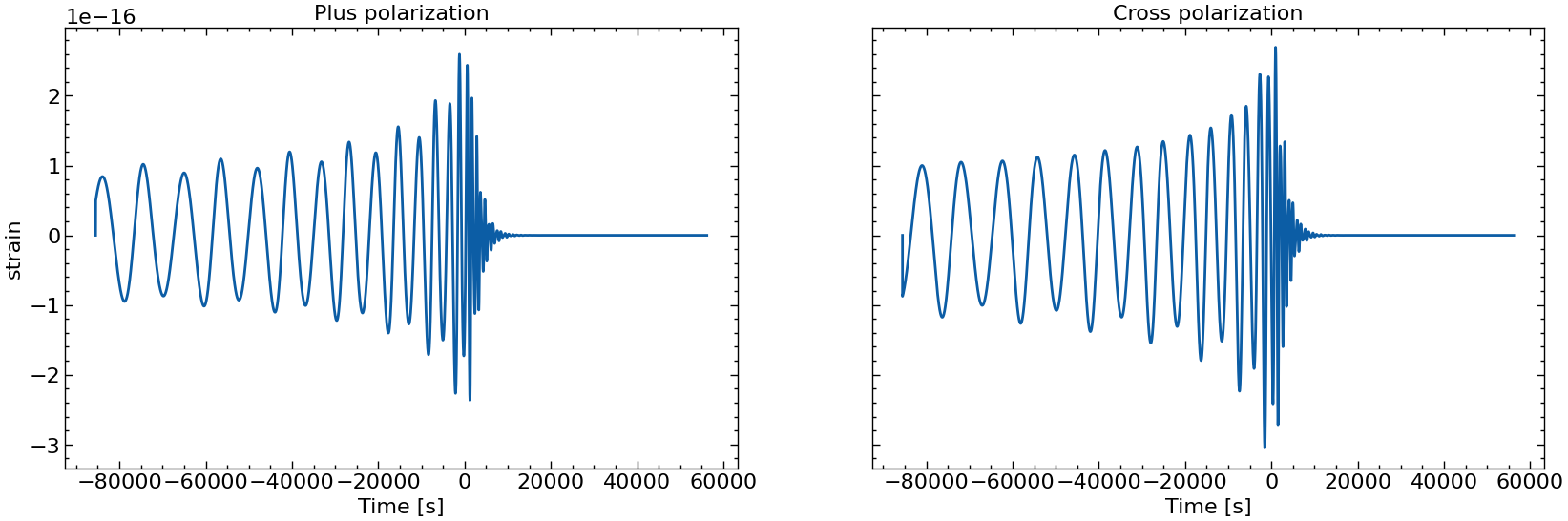
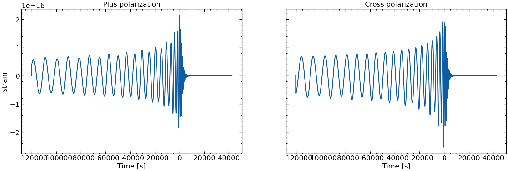
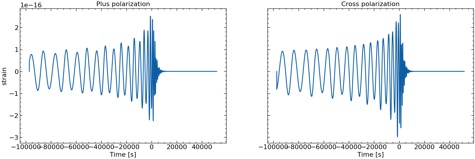
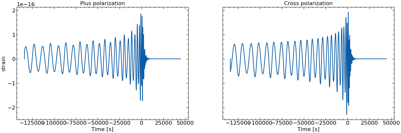
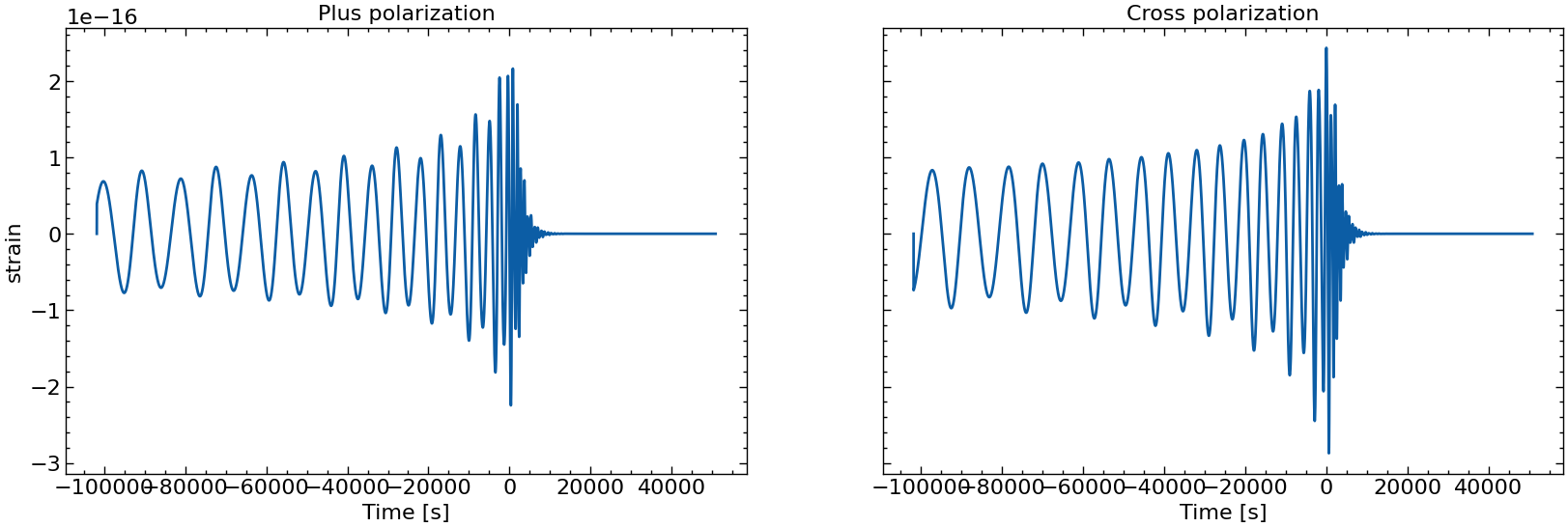
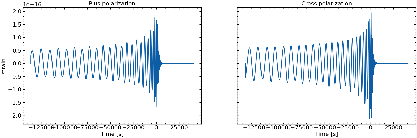
[18]:
# also plot them individually
for i in range(10):
    fig, axs = plt.subplots(1, 2, sharex=True, sharey=True, figsize=(2 * FIGSIZE[0], FIGSIZE[1]))
    axs[0].plot(times_batch[i], h_plus_batch[i])
    axs[1].plot(times_batch[i], h_cross_batch[i])

    axs[0].set_title("Plus polarization")
    axs[1].set_title("Cross polarization")
    #plt.legend()
    axs[0].set_xlabel("Time [s]")
    axs[1].set_xlabel("Time [s]")
    axs[0].set_ylabel("strain")
    plt.show()
Check against PhenomXPY
[19]:
from phenomxpy.phenomt.internals import pWF
from phenomxpy.phenomt.phenomt import IMRPhenomTHM as xpy_thm
[20]:
batch_idx = 3

m1_here = float(m1_batch[batch_idx])
m2_here = float(m2_batch[batch_idx])
chi1_here = float(chi1_batch[batch_idx])
chi2_here = float(chi2_batch[batch_idx])
distance = float(distance_batch[batch_idx])
inclination_here = float(inclination_batch[batch_idx])
psi_here = float(psi_batch[batch_idx])
phi_ref_here = float(phi_ref_batch[batch_idx])
[21]:
tic = time.time()
pwf = pWF(
        eta=m1_here * m2_here / (m1_here + m2_here) ** 2,
        s1=chi1_here,
        s2=chi2_here,
        f_min=f_min,
        f_ref=f_ref,
        total_mass=m1_here + m2_here,
        distance=distance,
        inclination=inclination_here,
        polarization_angle=psi_here,
        delta_t=delta_t,
        phi_ref=phi_ref_here,
    )

mode_array = None

xpy_wave_gen = xpy_thm(mode_array=mode_array, pWF_input=pwf)

xpy_plus, xpy_cross, xpy_times = xpy_wave_gen.compute_polarizations()

print(f"Time elapsed: {time.time() - tic} s")
Time elapsed: 5.61545205116272 s
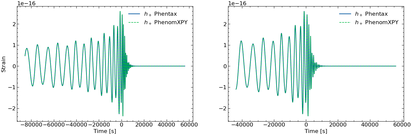
[22]:
fig, axs = plt.subplots(1, 2, figsize=(2 * FIGSIZE[0], FIGSIZE[1]))
axs[0].plot(times_batch[batch_idx][mask_batch[batch_idx]], h_plus_batch[batch_idx][mask_batch[batch_idx]], label=r'$h_+$ Phentax')
axs[0].plot(xpy_times, xpy_plus, lw=1.5, ls='--', label=r'$h_+$ PhenomXPY')
axs[0].legend()
axs[0].set_xlabel('Time [s]')
axs[0].set_ylabel('Strain')

# zoom on the end
axs[1].plot(times_batch[batch_idx][-10000:], h_plus_batch[batch_idx][-10000:], label=r'$h_+$ Phentax')
axs[1].plot(xpy_times[-10000:], xpy_plus[-10000:], lw=1.5, ls='--', label=r'$h_+$ PhenomXPY')
axs[1].legend()
axs[1].set_xlabel('Time [s]')

plt.show()
spline phenomxpy to compute the difference
Since the two code may return different time grids, we need to compare on the same one.
[23]:
from scipy.interpolate import Akima1DInterpolator
[24]:
times_here = times_batch[batch_idx][mask_batch[batch_idx]][:-1] # remove the very last point for the interpolation. it's zero anyways

spline = Akima1DInterpolator(xpy_times, xpy_plus)
xpy_new_times = spline(times_here)
[25]:
np.isclose(h_plus_batch[batch_idx][mask_batch[batch_idx]][:-1], xpy_new_times).all()
[25]:
np.True_