[1]:
from cantuccio import cornerplot

import numpy as np
import scipy
import matplotlib.pyplot as plt

import marimo as mo
Start generating some data
[2]:
def get_samples(means, vars, size):
    samples = []
    labels = []

    for i, (mu, var) in enumerate(zip(means, vars)):
        print(f"adding component {i}")
        _samples = scipy.stats.distributions.norm(mu, var).rvs(size)
        samples.append(_samples)
        labels.append(rf"$\mu_{i}$")

    return dict(zip(labels, np.stack(samples, axis=0)))
[3]:
mus = [5, 3, 10]

first_chain = get_samples(mus, [2, 1, 5], 1000)
adding component 0
adding component 1
adding component 2
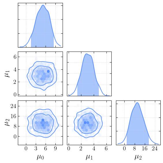
let’s see how they look
[4]:
_ = cornerplot(samples=first_chain)
plt.show()
We can now change the style…
[5]:
from cantuccio.core import OFFDIAG_MODES
styles = mo.ui.dropdown(options=OFFDIAG_MODES, value='hexbin+kde')
styles
[5]:
[6]:
_ =cornerplot(samples=first_chain, offdiag_mode=styles.value)
plt.show()

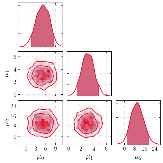
… change the KDE estimation method to use KDEpy’s FFTKDE…
[7]:
_fig, _axs =cornerplot(samples=first_chain, offdiag_mode=styles.value, kde_kwargs={"fast": False})
_ =cornerplot(samples=first_chain, offdiag_mode=styles.value, kde_kwargs={"fast": True}, fig=_fig, axes=_axs, colors=["red"])
plt.show()
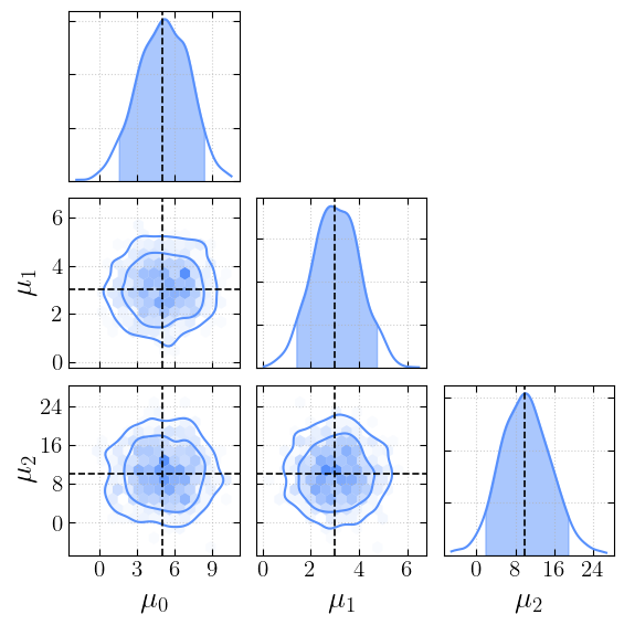
… add the true values…
[8]:
truths = dict(zip(first_chain.keys(), mus))
[9]:
_ = cornerplot(samples=first_chain, truths=truths)
plt.show()
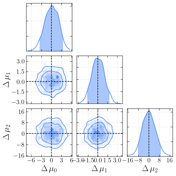
… plot the difference between data and injection …
[10]:
_ = cornerplot(samples=first_chain, truths=truths, plot_delta=True)
plt.show()
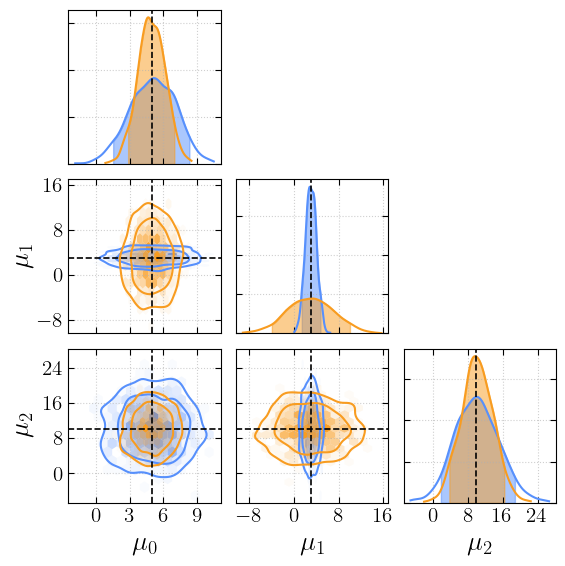
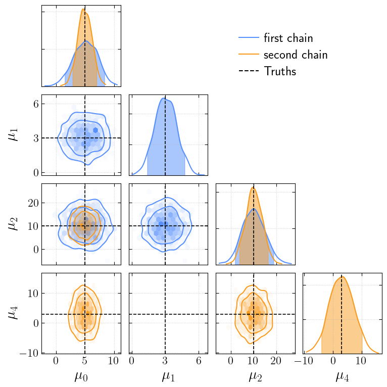
… add a second chain …
[11]:
second_chain = get_samples(mus, [1.2, 4.1, 3.7], 1000)
adding component 0
adding component 1
adding component 2
[12]:
_ = cornerplot(samples=[first_chain, second_chain], truths=truths)
plt.show()
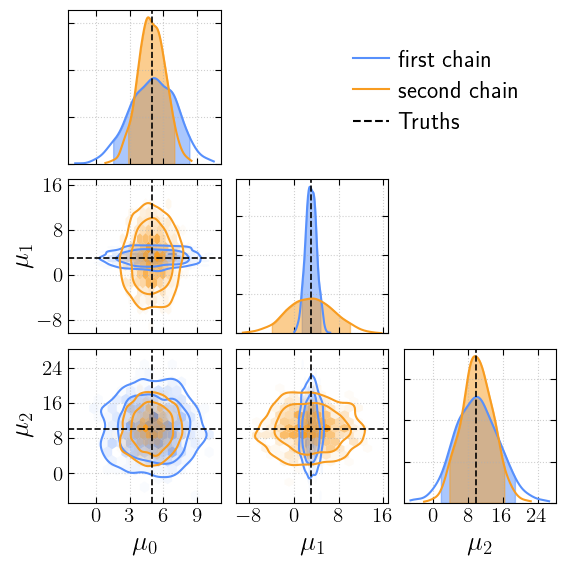
… and label them …
[13]:
_ = cornerplot(samples=[first_chain, second_chain], truths=truths, labels=['first chain', 'second chain'])
plt.show()
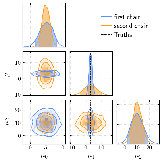
If the ticks overlap, we can decrease their number
[14]:
_ = cornerplot(samples=[first_chain, second_chain], truths=truths, labels=['first chain', 'second chain'], n_ticks=3)
plt.show()
Chains do not have to share the same parameters, but we can still plot them together
[15]:
_second_chain = second_chain.copy()
_second_chain[r"$\mu_4$"] = _second_chain[r"$\mu_1$"]

_second_chain.pop(r"$\mu_1$")

_truths = truths.copy()
_truths[r"$\mu_4$"] = truths[r"$\mu_1$"]

_ = cornerplot(samples=[first_chain, _second_chain], truths=_truths, labels=['first chain', 'second chain'], n_ticks=3)
plt.show()
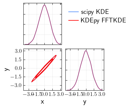
Now let’s see how the corner plot looks for higly correlated parameters under the two KDE estimation methods.
[16]:
cov = np.array([[1, 0.99], [0.99, 1]])
x, y = np.random.multivariate_normal([0, 0], cov, size=1000).T
samples = {"x": x, "y": y}
[17]:
_fig, _axs = cornerplot(samples=samples, offdiag_mode='kde', labels='scipy KDE', )
_ = cornerplot(samples=samples, offdiag_mode='kde', kde_kwargs={"fast": True, "alpha": 0.5}, fig=_fig, axes=_axs, colors="red", labels='KDEpy FFTKDE')
plt.show()
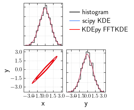
And against the histogram:
[18]:
_fig, _axs = cornerplot(samples=samples, offdiag_mode='kde', diag_mode='hist', colors="k", labels='histogram')
_fig, _axs = cornerplot(samples=samples, offdiag_mode='kde', kde_kwargs={"fast": False, "alpha": 0.5}, labels='scipy KDE', fig=_fig, axes=_axs)
_fig, _axs = cornerplot(samples=samples, offdiag_mode='kde', kde_kwargs={"fast": True, "alpha": 0.5}, fig=_fig, axes=_axs, colors="red", labels='KDEpy FFTKDE')

plt.show()
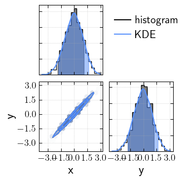
Using KDEs or histograms can provide slightly different estimated credible intervals.
[19]:
_fig, _axs = cornerplot(samples=samples, diag_mode='hist', colors="k", labels='histogram')
_fig, _axs = cornerplot(samples=samples, labels='KDE', fig=_fig, axes=_axs)

plt.show()
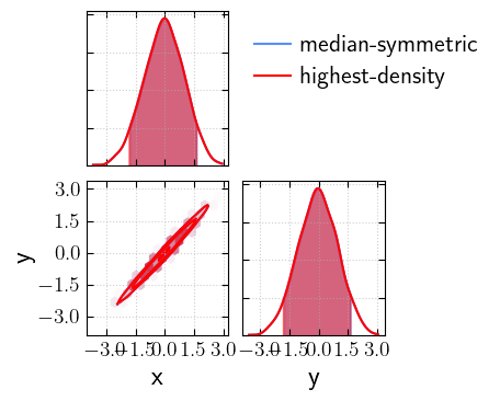
Median-symmetric vs highest-density credible intervals
For symmetric, unimodal distributions, the two methods give the same result. However, for skewed or multimodal distributions, they can differ significantly:
[20]:
_fig, _axs = cornerplot(samples=samples, statistic="median", labels='median-symmetric')
_ = cornerplot(samples=samples, statistic="hdi", labels='highest-density', fig=_fig, axes=_axs, colors="red")
plt.show()
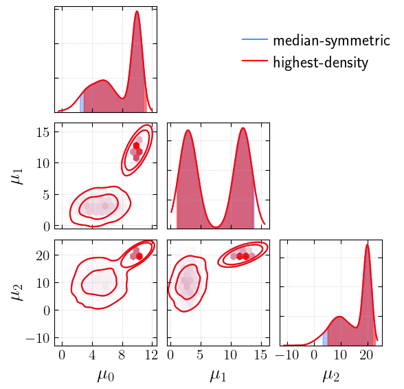
[21]:
# let's generate multimodal samples
multi_mus = [5, 3, 10]
multi_vars = [2, 1, 5]
component_1 = get_samples(multi_mus, multi_vars, 1000)
multi_mus = [10, 12, 20]
multi_vars = [0.2, 1, 0.5]
component_2 = get_samples(multi_mus, multi_vars, 1000)

multi_samples = {k: np.concatenate([component_1[k], component_2[k]]) for k in component_1.keys()}
adding component 0
adding component 1
adding component 2
adding component 0
adding component 1
adding component 2
[22]:
_fig, _axs = cornerplot(samples=multi_samples, statistic="median", labels='median-symmetric')
_ = cornerplot(samples=multi_samples, statistic="hdi", labels='highest-density', fig=_fig, axes=_axs, colors="red")
plt.show()
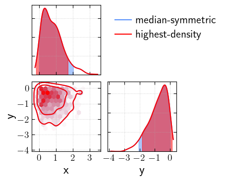
[23]:
# now let's try with a skewed distribution
skewed_samples_x = scipy.stats.distributions.skewnorm(a=10).rvs(size=1000)
skewed_samples_y = scipy.stats.distributions.skewnorm(a=-10).rvs(size=1000)
skewed_samples = {"x": skewed_samples_x, "y": skewed_samples_y}
[24]:
_fig, _axs = cornerplot(samples=skewed_samples, statistic="median", labels='median-symmetric')
_ = cornerplot(samples=skewed_samples, statistic="hdi", labels='highest-density', fig=_fig, axes=_axs, colors="red")
plt.show()
We can also overlay a covariance matrix ellipse on top of our corner plot if we have it available:
[25]:
new_mus = [5, 3, 10]
new_vars = np.array([2, 1, 5])

new_chain = get_samples(new_mus, new_vars, 1000)
adding component 0
adding component 1
adding component 2
[26]:
from cantuccio.core import overlay_covariance
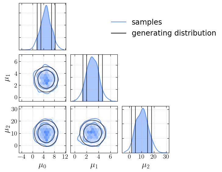
[27]:
_fig, _axs = cornerplot(samples=new_chain, contour_levels=[0.68, 0.90], labels='samples')
new_cov = np.diag(new_vars**2)
# Pass credible masses via `levels` (matching `contour_levels`) so the FIM
# ellipses line up with the corner contours. `num_sigmas` instead draws
# fixed-radius ellipses: a "1 sigma" ellipse encloses only 39% of the 2D
# mass, not the 68% that 1 sigma covers in 1D, so it would look too small.
_fig = overlay_covariance(_fig, new_cov, means=new_mus, plot_1d=True, colors='k', levels=[0.68, 0.90],  label='generating distribution')

plt.show()